We will simulate the effects of monetary policy on an economy using a simplified model.
The main variables are:
- Interest Rate (r):
Set by the central bank. - Inflation Rate (π):
Determined by economic conditions and influenced by monetary policy. - Output Gap (Y):
The difference between actual output and potential output, affected by interest rate changes.
This simulation will follow the logic of the Taylor Rule, a common monetary policy guideline:
$$
r = r^* + \phi_\pi (\pi - \pi^*) + \phi_Y Y
$$
- $(r^*)$ is the neutral interest rate.
- $(\pi^*)$ is the target inflation rate.
- $(\phi_\pi) and (\phi_Y)$ are policy reaction coefficients for inflation and output gap.
Python Implementation
Below is the $Python$ code to simulate the impact of monetary policy adjustments on inflation and the output gap over time.
1 | import numpy as np |
Explanation of the Code
- Model Setup:
- The neutral interest rate $(r^*)$, target inflation rate $(\pi^*)$, and policy reaction coefficients $(\phi_\pi$, $\phi_Y)$ are defined.
- Simulation Loop:
- The interest rate is updated using the Taylor Rule.
- The output gap and inflation rate are updated based on the interest rate, reflecting the dynamics of monetary policy.
- Visualization:
- The results for inflation, output gap, and interest rate over time are plotted.
Expected Results
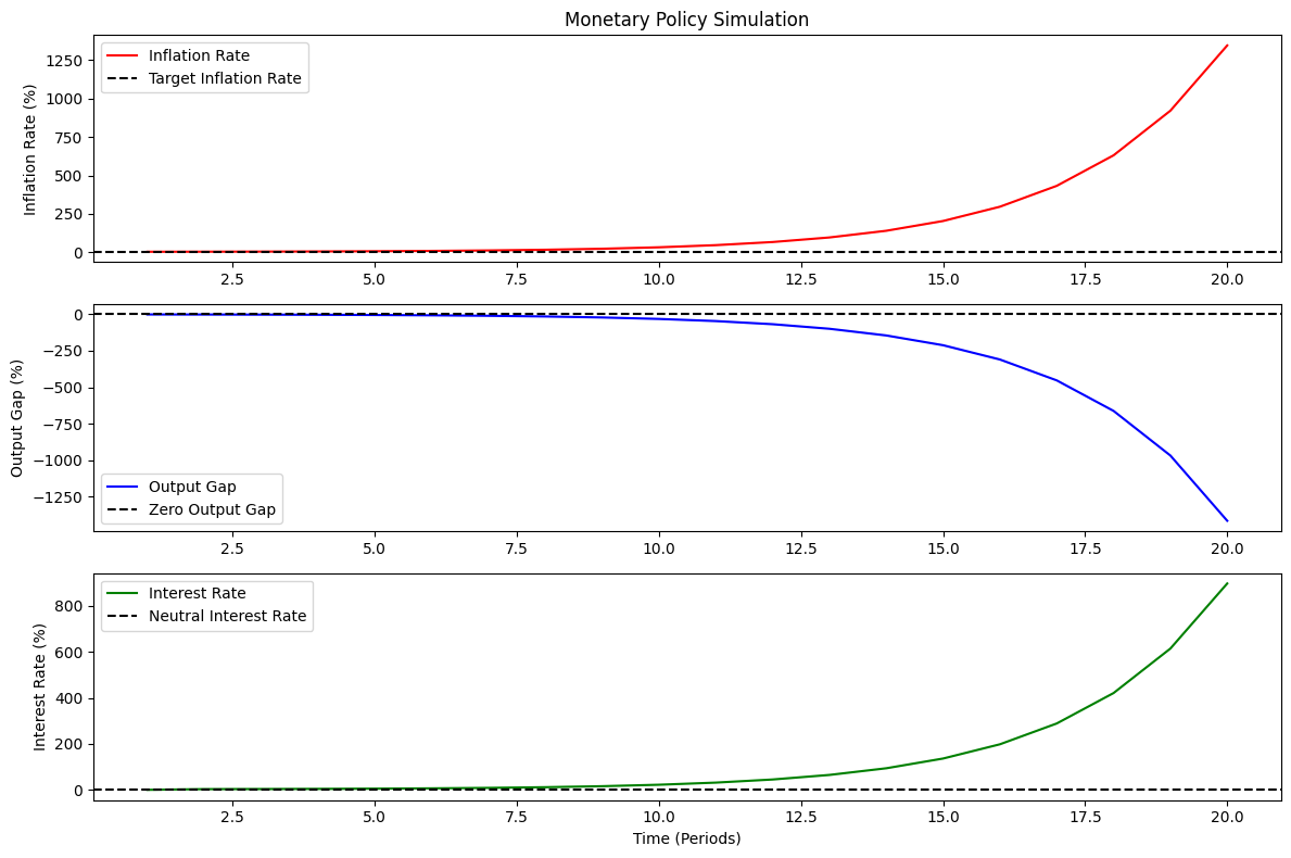
- Inflation Rate:
Gradually converges toward the target rate $(\pi^* = 2%)$. - Output Gap:
Oscillates and eventually stabilizes around zero. - Interest Rate:
Adjusts dynamically based on the Taylor Rule to stabilize inflation and output.
The graphs will visually illustrate these dynamics, helping to understand how monetary policy impacts an economy over time.