今回は、線形で分類できないデータを分類してみます。
円形データの生成
現実のデータではなく、scikit-learnのmake_circlesを使って、円形に散布するデータを生成します。
[Google Colaboratory]
1
2
3
4
5
6
| from sklearn.datasets import make_circles
X_circle, y_circle = make_circles(random_state=42, n_samples=100, noise=0.1, factor=0.3)
plt.scatter(X_circle[:, 0], X_circle[:, 1], c=y_circle)
plt.show()
|
[実行結果]
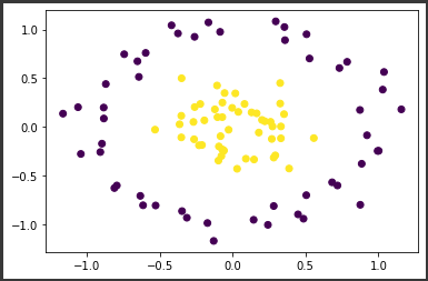
上図のように、線形では分類できそうもない、円の中に円があるようなデータが生成されました。
複数のモデルを定義
複数のモデルを構築するために、それぞれのモデルを辞書型で定義します。
[Google Colaboratory]
1
2
3
4
5
6
| models = {"Logistic Regression":LogisticRegression(),
"Linear SVM":LinearSVC(random_state=0),
"Kernel SVM":SVC(kernel="rbf",random_state=0),
"K Neighbors":KNeighborsClassifier(),
"Decision Tree":DecisionTreeClassifier(max_depth=3,random_state=0),
"Random Forest":RandomForestClassifier(max_depth=3,random_state=0)}
|
モデル構築・決定境界の可視化
定義した辞書内容をもとに、各モデルの構築と決定境界の可視化をまとめて行います。
[Google Colaboratory]
1
2
3
4
5
6
7
8
9
10
11
12
13
14
15
16
| import matplotlib.gridspec as gridspec
import itertools
gs = gridspec.GridSpec(2, 3)
fig = plt.figure(figsize=(12, 6))
for model_name, num in zip(models.keys(), itertools.product([0, 1, 2],repeat=2)):
model = models[model_name].fit(X_circle,y_circle)
ax = plt.subplot(gs[num[0], num[1]])
fig = plot_decision_regions(X_circle, y_circle,clf=model)
plt.title(model_name)
plt.tight_layout()
plt.show()
|
[実行結果]
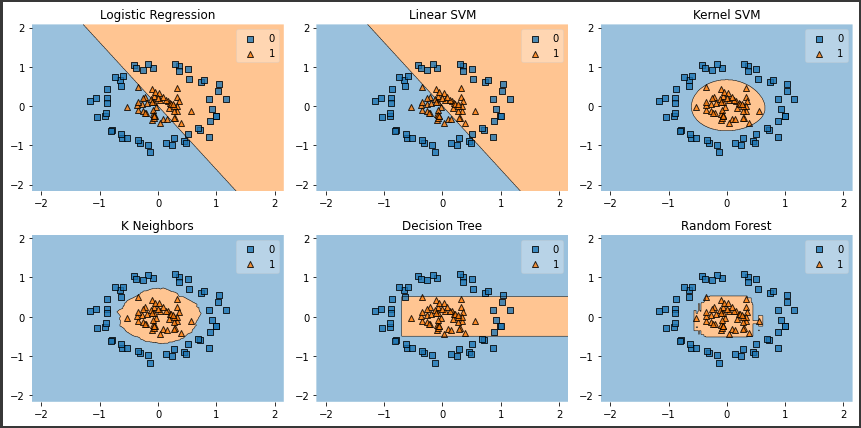
それぞれのモデルの決定境界を一括で可視化できました。
上記の図から、ロジスティック回帰や線形SVMのような線形系アルゴリズムでは、今回のデータセットには全く対応できていないことが把握できます。
一方、カーネルSVM、K近傍法、ランダムフォレストでは適切に分類することができています。
アルゴリズムを選択する際には、まずデータセットの散布状況を確認し線形分離できそうかどうかを確認するのがよさそうです。