Python × AI [クラスタリング] - k-means++

k-meansのパラメータを調整してクラスタリングを実行し、結果がどうかわるかを見てみます。

k-means++

初期パラメータのinitパラメータをrandomからk-means++にしてクラスターの初期位置を変更します。(1行目)

randomの場合は、クラスターセンターがランダムに設置されますが、k-meansの場合は、初期のクラスターセンターを互いに離れた位置に配置します。

k-means++に設定することにより、より効率的で一貫性のある結果が得られるようになります。

クラスタリングを行い、グラフ化を行います。

[Google Colaboratory]

model = KMeans(n_clusters=3, random_state=0, init="k-means++")
cls_data = df_iris.copy()
model.fit(cls_data)
cluster = model.predict(cls_data)
cls_data["cluster"] = cluster
sns.pairplot(cls_data, hue="cluster")

[実行結果]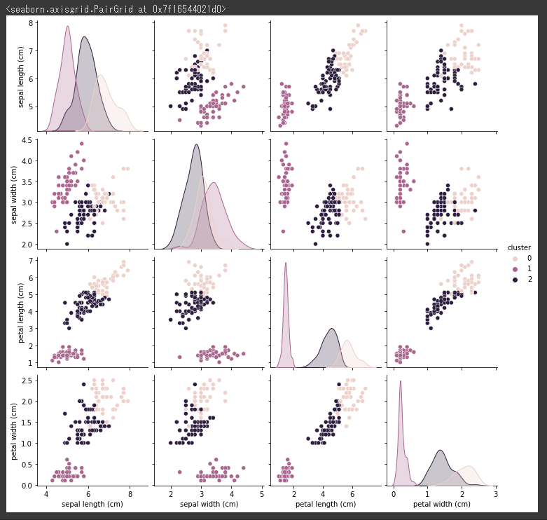

調整ランド指数(ARI)

クラスタリングした結果の調整ランド指数(ARI)を算出します。

[Google Colaboratory]

ari = "ARI: {:.2f}".format(adjusted_rand_score(iris.target, cls_data["cluster"]))
print(ari)

[実行結果]

結果は0.73と前回と同じ結果になりました。

結果は改善しませんでしたが、k-means++はランダムより収束が早いという特徴があるため、基本的にk-means++を使うことをお勧めします。

（initパラメータを指定しなければデフォルトでk-means++となります。）

クラスタ数の変更

クラスタ数を3から2に変更してみます。

クラスタリング、グラフ化、調整ランド指数の算出まで一気に実行します。

[Google Colaboratory]

model = KMeans(n_clusters=2, random_state=0)
cls_data = df_iris.copy()
cls_data["cluster"] = model.fit_predict(cls_data)
sns.pairplot(cls_data, hue="cluster")
print("ARI: {:.2f}".format(adjusted_rand_score(iris.target, cls_data["cluster"])))

[実行結果]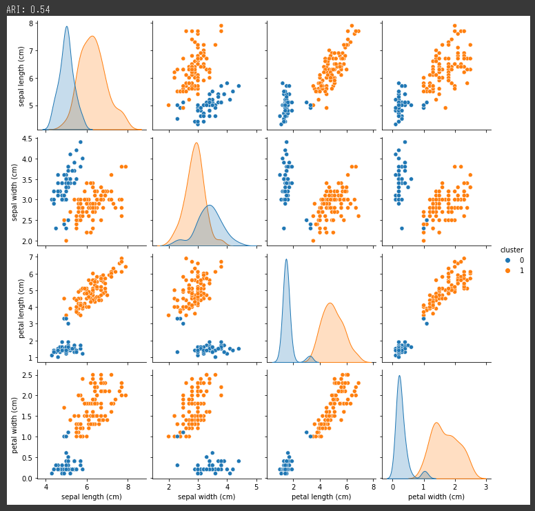

グラフに表示される色の種類から、2つのクラスタ（グループ）にまとめられたことが分かります。

調整ランド指数(ARI)は0.54と下がってしまったので、今回実施したクラスタ数2よりもクラスタ数3の方が精度が高かったことが分かります。

次回は、適切なクラスタ数を探索する方法を試してみます。