Natural Language Processing with Disaster Tweetsr に関する3回目の記事です。
Natural Language Processing with Disaster Tweets
今回は単語ごとの解析を行います。
単語解析
ツイートを単語ごとに分割する関数を定義します。
引数のtargetには災害関連(=1)か災害に関係ない(=0)かを渡します。
[ソース]
1
2
3
4
5
6
7
def create_corpus(target): corpus=[] for x in tweet[tweet['target']==target]['text'].str.split(): for i in x: corpus.append(i) return corpus
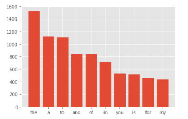
災害に関係のないツイート(target=0)を単語ごとに分割し、出現頻度が多い順にグラフ化します。
[ソース]
1
2
3
4
5
6
7
8
9
10
11
corpus = create_corpus(0) dic=defaultdict(int) for word in corpus: if word in stop: dic[word] += 1 top = sorted(dic.items(), key=lambda x:x[1], reverse=True)[:10] x,y=zip(*top) plt.bar(x,y)
[結果]
the、a、to という冠詞、前置詞の出現が多いようです。
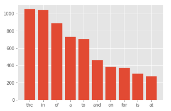
次に災害に関係のあるツイート(target=1)を単語ごとに分割し、出現頻度が多い順にグラフ化します。
[ソース]
1
2
3
4
5
6
7
8
9
10
11
12
corpus=create_corpus(1) dic=defaultdict(int) for word in corpus: if word in stop: dic[word]+=1 top=sorted(dic.items(), key=lambda x:x[1],reverse=True)[:10] x,y=zip(*top) plt.bar(x,y)
[結果]
こちらもthe、in、of という冠詞、前置詞の出現が多いようです。
句読点
今度は句読点について調べていきます。
string.punctuation (6行目)は、英数字以外のアスキー文字(句読点含む)を表します。
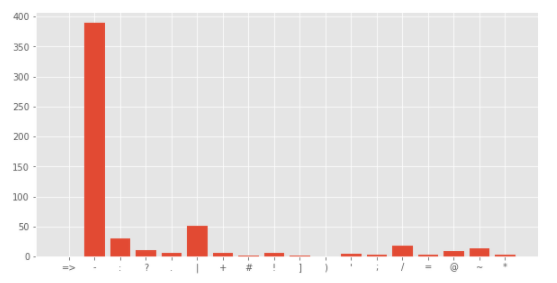
災害に関係のあるツイートの句読点出現回数をグラフで表示します。
[ソース]
1
2
3
4
5
6
7
8
9
10
11
12
plt.figure(figsize=(10,5)) corpus = create_corpus(1) dic = defaultdict(int) import string special = string.punctuation for i in (corpus): if i in special: dic[i] += 1 x,y = zip(*dic.items()) plt.bar(x,y)
[結果]
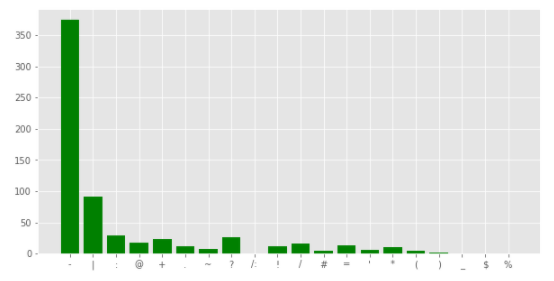
災害に関係のないツイートの句読点出現回数をグラフで表示します。
[ソース]
1
2
3
4
5
6
7
8
9
10
11
12
13
plt.figure(figsize=(10,5)) corpus = create_corpus(0) dic = defaultdict(int) import string special = string.punctuation for i in (corpus): if i in special: dic[i] += 1 x, y = zip(*dic.items()) plt.bar(x,y,color='green')
[結果]
どちらも1番目が-(ハイフン) 、2番目が|(パイプ) と同じですが、3番目は:(コロン)と?(クエスチョン) と少し違いがあるようです。
共通する単語(ストップワード以外)
最後にストップワードを含まない共通する単語を調べます。
ストップワードとは、自然言語を処理するにあたって処理対象外とする単語のことです。
「at」「of」などの前置詞や、「a」「an」「the」などの冠詞、「I」「He」「She」などの代名詞がストップワードとされます。
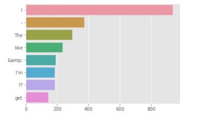
ストップワードに含まれない単語を抽出し、グラフ化します。
[ソース]
1
2
3
4
5
6
7
8
9
10
counter = Counter(corpus) most = counter.most_common() x=[] y=[] for word,count in most[:40]: if (word not in stop) : x.append(word) y.append(count) sns.barplot(x=y, y=x)
[結果]
まだハイフンやアンパサンドなどがあるので、さらにデータクレンジングをする必要がありそうです。
N-gram解析
N-gram解析 とは、対象となるテキストの中で、連続するN個の表記単位(gram)の出現頻度を求める手法です。
そうすることによって、テキスト中の任意の長さの表現の出現頻度パターンなどを知ることができるようになります。
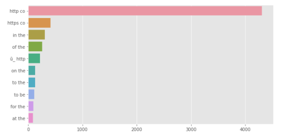
N=2(bigram)として、N-gram解析を行います。
[ソース]
1
2
3
4
5
6
7
8
9
10
11
12
def get_top_tweet_bigrams(corpus, n=None): vec = CountVectorizer(ngram_range=(2, 2)).fit(corpus) bag_of_words = vec.transform(corpus) sum_words = bag_of_words.sum(axis=0) words_freq = [(word, sum_words[0, idx]) for word, idx in vec.vocabulary_.items()] words_freq =sorted(words_freq, key = lambda x: x[1], reverse=True) return words_freq[:n] plt.figure(figsize=(10,5)) top_tweet_bigrams=get_top_tweet_bigrams(tweet['text'])[:10] x,y=map(list,zip(*top_tweet_bigrams)) sns.barplot(x=y,y=x)
[結果]
これに関しても、URLに関するものが多かったり、前置詞・冠詞の組み合わせが多かったりと、まだまだデータクレンジングが必要そうです。
というわけで、次回はデータクレンジングを行っていきます。